Quickstart

In this tutorial, we will show how to solve a famous optimization problem, minimizing the Rosenbrock function, in simplenlopt. First, let’s define the Rosenbrock function and plot it:

\[f(x, y) = (1-x)^2+100(y-x^2)^2\]

import numpy as np

def rosenbrock(pos):

    x, y = pos
    return (1-x)**2 + 100 * (y - x**2)**2

xgrid = np.linspace(-2, 2, 500)
ygrid = np.linspace(-1, 3, 500)

X, Y = np.meshgrid(xgrid, ygrid)

Z = (1 - X)**2 + 100 * (Y -X**2)**2

x0=np.array([-1.5, 2.25])
f0 = rosenbrock(x0)

#Plotly not rendering correctly on Readthedocs, but this shows how it is generated! Plot below is a PNG export
import plotly.graph_objects as go
fig = go.Figure(data=[go.Surface(z=Z, x=X, y=Y, cmax = 10, cmin = 0, showscale = False)])
fig.update_layout(
    scene = dict(zaxis = dict(nticks=4, range=[0,10])))
fig.add_scatter3d(x=[1], y=[1], z=[0], mode = 'markers', marker=dict(size=10, color='green'), name='Optimum')
fig.add_scatter3d(x=[-1.5], y=[2.25], z=[f0], mode = 'markers', marker=dict(size=10, color='black'), name='Initial guess')
fig.show()

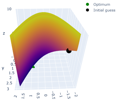
The crux of the Rosenbrock function is that the minimum indicated by the green dot is located in a very narrow, banana shaped valley with a small slope around the minimum. Local optimizers try to find the optimum by searching the parameter space starting from an initial guess. We place the initial guess shown in black on the other side of the banana.

In simplenlopt, local optimizers are called by the minimize function. It requires the objective function and a starting point. The algorithm is chosen by the method argument. Here, we will use the derivative-free Nelder-Mead algorithm. Objective functions must be of the form f(x, ...) where x represents a numpy array holding the parameters which are optimized.

import simplenlopt

def rosenbrock(pos):

    x, y = pos
    return (1-x)**2 + 100 * (y - x**2)**2

res = simplenlopt.minimize(rosenbrock, x0, method = 'neldermead')
print("Position of optimum: ", res.x)
print("Function value at Optimum: ", res.fun)
print("Number of function evaluations: ", res.nfev)

Position of optimum:  [0.99999939 0.9999988 ]
Function value at Optimum:  4.0813291938703456e-13
Number of function evaluations:  232

The optimization result is stored in a class whose main attributes are the position of the optimum and the function value at the optimum. The number of function evaluations is a measure of performance: the less function evaluations are required to find the minimum, the faster the optimization will be.

Next, let’s switch to a derivative based solver. For better performance, we also supply the analytical gradient which is passed to the jac argument.

def rosenbrock_grad(pos):

    x, y = pos
    dx = 2 * x -2 - 400 * x * (y-x**2)
    dy = 200 * (y-x**2)

    return dx, dy

res_slsqp = simplenlopt.minimize(rosenbrock, x0, method = 'slsqp', jac = rosenbrock_grad)
print("Position of optimum: ", res_slsqp.x)
print("Function value at Optimum: ", res_slsqp.fun)
print("Number of function evaluations: ", res_slsqp.nfev)

Position of optimum:  [1. 1.]
Function value at Optimum:  1.53954903146237e-20
Number of function evaluations:  75

As the SLSQP algorithm can use gradient information, it requires less function evaluations to find the minimum than the derivative-free Nelder-Mead algorithm.

Unlike vanilla NLopt, simplenlopt automatically defaults to finite difference approximations of the gradient if it is not provided:

res = simplenlopt.minimize(rosenbrock, x0, method = 'slsqp')
print("Position of optimum: ", res.x)
print("Function value at Optimum: ", res.fun)
print("Number of function evaluations: ", res.nfev)

Position of optimum:  [0.99999999 0.99999999]
Function value at Optimum:  5.553224195710645e-17
Number of function evaluations:  75

C:\Users\danie\.conda\envs\simplenlopt_env\lib\site-packages\simplenlopt\_Core.py:178: RuntimeWarning: Using gradient-based optimization, but no gradient information is available. Gradient will be approximated by central difference. Consider using a derivative-free optimizer or supplying gradient information.
  warn('Using gradient-based optimization'

As the finite differences are not as precise as the analytical gradient, the found optimal function value is higher than with analytical gradient information. In general, it is aways recommended to compute the gradient analytically or by automatic differentiation as the inaccuracies of finite differences can result in wrong results and bad performance.

For demonstration purposes, let’s finally solve the problem with a global optimizer. Like in SciPy, each global optimizer is called by a dedicated function such as crs() for the Controlled Random Search algorithm. Instead of a starting point, the global optimizers require a region in which they seek to find the minimum. This region is provided as a list of (lower_bound, upper_bound) for each coordinate.

bounds = [(-2., 2.), (-2., 2.)]
res_crs = simplenlopt.crs(rosenbrock, bounds)
print("Position of optimum: ", res_crs.x)
print("Function value at Optimum: ", res_crs.fun)
print("Number of function evaluations: ", res_crs.nfev)

Position of optimum:  [1.00000198 1.00008434]
Function value at Optimum:  6.45980535135501e-07
Number of function evaluations:  907

Note that using a global optimizer is overkill for a small problem like the Rosenbrock function: it requires many more function evaluations than a local optimizer. Global optimization algorithms shine in case of complex, multimodal functions where local optimizers converge to local minima instead of the global minimum. Check the Global Optimization page for such an example.